1. Blackwell SM_100a Tensor Core Architecture
2025-02-14
1.1. Tensor Memory
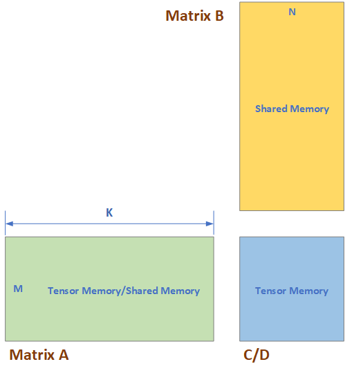
Blackwell architecture introduced new features like Tensor Memory to relief the pressure of Shared memory and Vector Register. Such that the matrices can be read from Tensor Memory and Shared Memory, instead of from Vector Register. The matrices are stored as shown in Table 8 and Table 8 Tensor Core Matrix Storage {#table-matrix-storage}
| Matrix Type | Memory |
|---|---|
| A | Tensor Memory OR Shared Memory |
| B | Shared Memory |
| D | Tensor Memory |
| Sparse Meta Data | Tensor Memory |
| A-Scale / B-Scale | Tensor Memory |
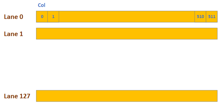
Tensor Memory is a 128*512 Dwords memory for each Stream Multi-Processor (SM), and it has 128 lanes while each lane has 512 Dwords, shown as in Figure 2. These 128 lanes can be accessed simultaneously and thus the read or write bandwidth should be 128 Dwords/cycle.
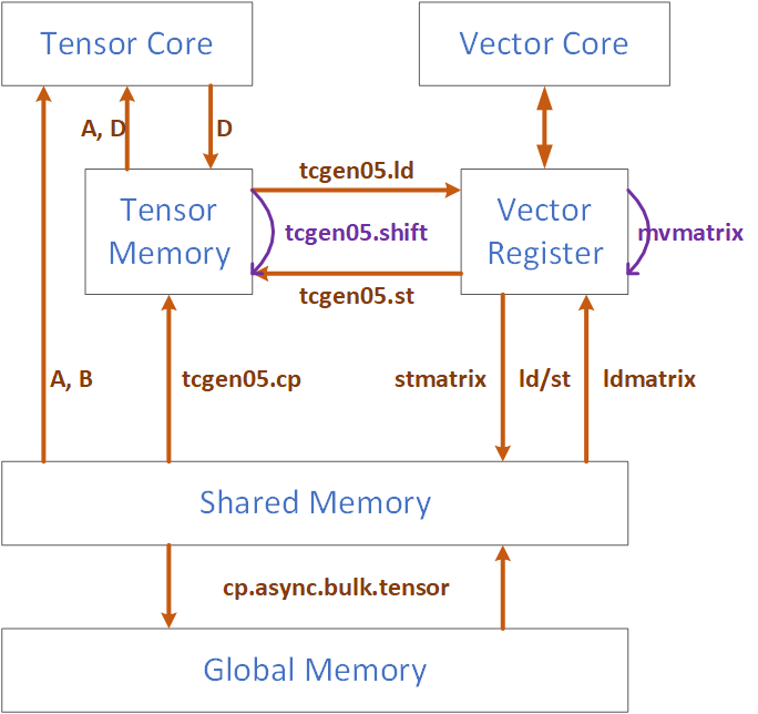
Data can be moved between Tensor Memory and Vector Register, and from Shared Memory to Tensor Memory. These data movement instructions are denoted in Figure 3.
1.1.1. Tcgen05.shift
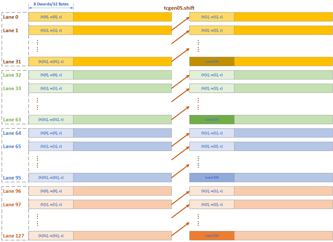
Tensor Memory has a shift operation which enables the acceleration and data reuse of convolution, which would be described detailly in Section 3.2. In tcgen05.shift, the data of each lane would be shifted to next lane, except the last lane, which is Lane[0] in Figure 4.
1.1.2. Tensor Memory Architecture
A possible architecture of Tensor Memory is shown in Figure 5:
- For each 32-thread, or for each Tensor Core, or in each CU, the Tensor Memory has 8 standard alone banks and each bank’s bandwidth is 32 Dwords for 1 Dword/thread, and the depth is 64.
- There are 4 such groups, each group for 32-thread/Tensor Core, thus 32 banks in total for Tensor Memory.
- Inside of each Tensor Memory group, Bank n contains the Column 8*col+n with col=[0,1, … 63].
With this design, it is possible to finish the tcgen05.shift in 1 cycle. There could be different architecture for Tensor Memory, as there is a balance between speed and resource overhead. For example, 4 banks and each bank 128 entries, and the tcgen05.shift takes 2 cycle in this case.
1.2. Convolution
1.2.1. Algorithm
Blackwell improve the efficiency of convolution operation by reusing the Activation data in Tensor Memory. As shown in previous section, the data in Tensor Memory can be shifted by one lane, and this feature can be used to reuse the Activation data thus to relief the bandwidth of Shared Memory.
The original convolution operation with OH/H in the outer loop is shown in Algorithm 1, we will derive the Blackwell Convolution implementation from it.
Algorithm 1 Original Convolution with OH in Outer Loop
1
2
3
4
5
6
7
8
9
10
for (p=0; p<P; p++) // OH
  for (nq=0; nq<NQ; nq++) // N, OW
    {n, q} = F(nq)
    for (r=0; r<R; r++)
      for (s=0; s<S; s++)
        h = p * stride_H - pad_H + r * dilation_h;
        w = q * stride_W - pad_W + s * dilation_w;
        for (k=0; k<K; k++)
          for (c=0; c<C; c++)
            O[n][p][q][k] += A[n][h][w][c] * W[k][r][s][c];
We can map the Algorithm 1 to MMA operation shown in Algorithm 2. Up till now, we haven’t taken the Activation Data Reuse into consideration yet.
Algorithm 2 Convolution with OH in Outer Loop using MMA
1
2
3
4
5
6
7
8
9
10
11
12
13
14
15
16
17
18
19
20
21
22
23
24
25
26
27
28
29
30
31
32
33
34
////////////////////////////////////////////////////////////////////////////////
// Blackwell Convolution
// Outer Iteration at OH level
// Weight in MMA_A[MMA_M][MMA_K], Activation in MMA_B[MMA_K][MMA_N]
////////////////////////////////////////////////////////////////////////////////
for (p=0; p<P; p++)               // OH
  for (nq=0; nq<NQ; nq=nq+MMA_N)  // N, OW
    for (r=0; r<R; r++)
      for (s=0; s<S; s++)
        for (k=0; k<K; k=k+MMA_M)   // MMA_M=16 Kernel in one group
          for (c=0; c<C; c=c+MMA_K) // MMA_K=32 data in one channel

            for (mma_m=0; mma_m<MMA_M; mma_m++)   // Weight data in MMA_A
              for (mma_k=0; mma_k<MMA_K; mma_k++)
                MMA_A[mma_m][mma_k] = W[k+mma_m][r][s][c+mma_k]

            for (mma_n=0; mma_n<MMA_M; mma_n++)   // Input Activation data in MMA_B
              {n, q} = (nq + mma_n);
              for (mma_k=0; mma_k<MMA_K; mma_k++)
                h = p * stride_H - pad_H + r * dilation_h;
                w = q * stride_W - pad_W + s * dilation_w;
                MMA_B[mma_n][mma_k] = A[n][h][w][c+mma_k];

            for (mma_m=0; mma_m<MMA_M; mma_m++)   // OA data in C/D
              for (mma_n=0; mma_n<MMA_N; mma_n++)
                {n, q} = (nq + mma_n);
                MMA_C[mma_m][mma_n] = O[n][p][q][k+mma_m];

            MMA_D = MMA_A * MMA_B + MMA_C;

            for (mma_m=0; mma_m<MMA_M; mma_m++)   // Write OA data back
              for (mma_n=0; mma_n<MMA_N; mma_n++)
                {n, q} = (nq + mma_n);
                O[n][p][q][k+mma_m] = MMA_D[mma_m][mma_n];
We notice that with s++, most of the data in matrix B, MMA_B, can be reused. We can load MMA_N rows of Activation data into MMA_B matrix when s==0 at beginning, and reuse most of them with s++, only loading one new row from Shared Memory into Tensor Memory.
Algorithm 3 Convolution with OH in Outer Loop using MMA , reuse Activation Data
1
2
3
4
5
6
7
8
9
10
11
12
13
14
15
16
17
18
19
20
21
22
23
24
25
26
27
28
29
30
31
32
33
34
35
36
37
38
39
40
41
42
43
44
45
////////////////////////////////////////////////////////////////////////////////
// Blackwell Convolution
// Outer Iteration at OH level, reuse Act data in S direction
// Weight in MMA_A[MMA_M][MMA_K], Activation in MMA_B[MMA_K][MMA_N]
////////////////////////////////////////////////////////////////////////////////
for (p=0; p<P; p++)               // OH
  for (nq=0; nq<NQ; nq=nq+MMA_N)  // N, OW
    for (r=0; r<R; r++)
      for (k=0; k<K; k=k+MMA_M)   // MMA_M=16 Kernel in one group
        for (c=0; c<C; c=c+MMA_K) // MMA_K=32 data in one channel
          for (s=0; s<S; s++)     // Reuse Activation data in S direction

            for (mma_m=0; mma_m<MMA_M; mma_m++)   // Weight data in MMA_A
              for (mma_k=0; mma_k<MMA_K; mma_k++)
                MMA_A[mma_m][mma_k] = W[k+mma_m][r][s][c+mma_k]

            // Input Activation data in MMA_B
            if (s == 0) // The first channel is S direction, fetch all data
              for (mma_n=0; mma_n<MMA_N; mma_n++) // Input Activation data in MMA_B
                {n, q} = (nq + mma_n);
                for (mma_k=0; mma_k<MMA_K; mma_k++)
                  h = p * stride_H - pad_H + r * dilation_h;
                  w = q * stride_W - pad_W + s * dilation_w;
                  MMA_B[mma_n][mma_k] = A[n][h][w][c+mma_k];
            else // for (s=1; s<S; s++)
              for (mma_n=1; mma_n<MMA_N; mma_n++) // tcg05.shift
                MMA_B[mma_n] = MMA_B[mma_n-1];
              for (mma_n=0; mma_n<1; mma_n++) // mma_n=0 is new from IA
                {n, q} = (nq + mma_n);
                h = p * stride_H - pad_H + r * dilation_h;
                w = q * stride_W - pad_W + s * dilation_w;
                for (mma_k=0; mma_k<MMA_K; mma_k++)
                  MMA_B[mma_n][mma_k] = A[n][h][w][c+mma_k];

            for (mma_m=0; mma_m<MMA_M; mma_m++)   // OA data in C/D
              for (mma_n=0; mma_n<MMA_N; mma_n++)
                {n, q} = (nq + mma_n);
                MMA_C[mma_m][mma_n] = O[n][p][q][k+mma_m];

            MMA_D = MMA_A * MMA_B + MMA_C;

            for (mma_m=0; mma_m<MMA_M; mma_m++)   // Write OA data back
              for (mma_n=0; mma_n<MMA_N; mma_n++)
                {n, q} = (nq + mma_n);
                O[n][p][q][k+mma_m] = MMA_D[mma_m][mma_n];
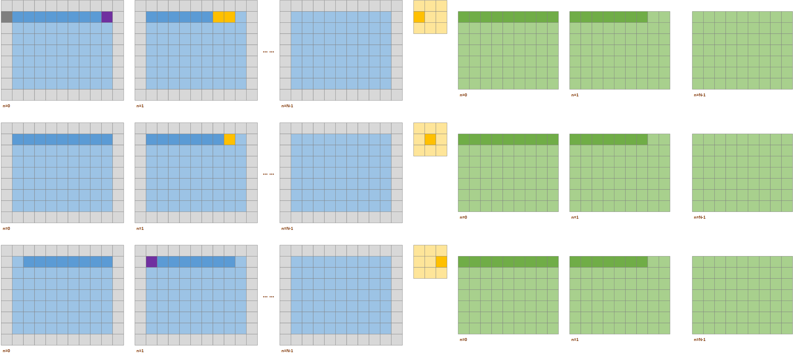
Take the convolution with Activation size (N, H=9, W=9, C), Weight Size (R=3, S=3, C, K) and Output Activation size (N, P=7, Q=9, K) shown in Figure 6 as an example. To generate the first 16 OA channels with p=0, which can be denoted as OA(n=0, p=0, q=[0:8], K) and OA(n=1, p=0, q=[p:6], K), marked as deep green color in Figure 6, the kernels may be convolved with the first 3 rows of the IA data. For the weight data W(r=1, S=[0:2], C, K), it will be multiplied with the 1st row of the IA data.
- For W(r=1, s=0, C, K), it will be operated with IA data IA(n=0, h=0, w=[-1:7], C) and IA(n=1, h=0, w=[-1:5], C). In which, the IA(n=0, h=0, w=-1, C) and IA(n=1, h=0, w=-1, C) are in the padded area.
- For W(r=1, s=1, C, K), it will be operated with IA data IA(n=0, h=0, w=[0:8], C) and IA(n=1, h=0, w=[0:6], C).
- For W(r=1, s=2, C, K), it will be operated with IA data IA(n=0, h=0, w=[1:9], C) and IA(n=1, h=0, w=[1:7], C). In which, the IA(n=0, h=0, w=9, C) is in the padding area.
The above three steps can be optimized by reusing most of the data of Input Activation. The first step is shown in Figure 7. While we need the IA data IA(n=0, h=0, w=[-1:7], C) and IA(n=1, h=0, w=[-1:5], C) for W(r=1, s=0, C, K), we load the IA data IA(n=0, h=0, w=[-1:8], C) and IA(n=1, h=0, w=[0:5], C) are loaded into Tensor Memory as shown in the left side of Figure 7 (a). As IA(n=0, h=0, w=-1, C) and IA(n=1, h=0, w=-1, C) are in padding area, they would be treated differently:
- For IA(n=0, h=0, w=-1, C), it is in the left padding area of the 1st image, it should be loaded into Tensor Memory and it is marked in grey color in the left side of Figure 7 (a).
- For IA(n=1, h=0, w=-1, C), it is in the left padding area of the 2nd image, it should not be loaded into Tensor Memory, instead, we should mask some other data and replace them with the padding value which is 0 here. In the left side of Figure 7 (a), we mark IA(n=0, h=0, w=8, C) in purple color as W(r=1, s=0, C, K) will not operate with this channel. For this purple row:
- We can replace the data in purple row with the padding value which is 0 here.
- We can skip to write the corresponding row of D back into Tensor Memory, or write 0 back to Tensor Memory. The corresponding row of D is also marked in gray color in right side of Figure 7 (a).
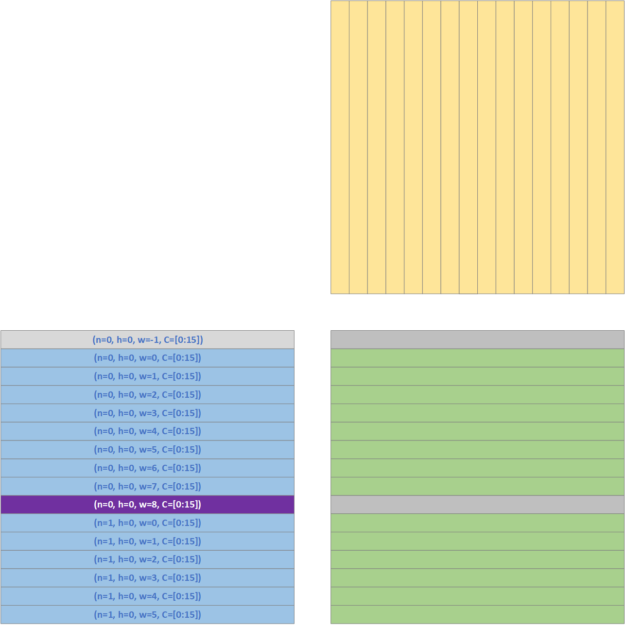

After finishing the computation of W(r=1, s=0, C, K), we do not need to load all the IA data for W(r=1, s=1, C, K). Show in Figure 7 (b), we shift the IA data one lane, then IA(n=0, h=0, w=-1, C) would be discarded, and we only need to load IA(n=1, h=0, w=6, C) in this case. As none of the rows are from the padding area, we do not need to mask out any rows in this case.
Similarly, after finishing the computation of W(r=1, s=1, C, K), we can reuse most of the IA data for W(r=1, s=2, C, K). Show in Figure 7 (b), we shift the IA data one lane, then IA(n=0, h=0, w=0, C) would be discarded, and we only need to load IA(n=1, h=0, w=7, C) in this case. As W(r=1, s=2, C, K) needs IA(n=0, h=0, w=9, C) which is in the right padding area, this data is not loaded into memory and we need to mask the corresponding channel IA(n=1, h=0, w=0, C) which is not required by W(r=1, s=2, C, K) and it is marked in purple color in the right side of Figure 7 (b).
1.2.2. Instruction
Blackwell provides MMA instruction designed for convolution specifically, which is shown in Table 9. Table 9 MMA Instruction for Convolution
1
2
3
4
5
6
7
8
9
10
11
12
13
14
15
16
// 3. Convolution MMA for floating-point type without block scaling:

tcgen05.mma.cta_group.kind.collector_usage [d-tmem],  a-desc,  b-desc, idesc,
                                          { disable-output-lane }, enable-input-d {, scale-input-d};

tcgen05.mma.cta_group.kind{.ashift}.collector_usage [d-tmem], [a-tmem], b-desc, idesc,
                                          { disable-output-lane }, enable-input-d {, scale-input-d};

tcgen05.mma.cta_group.kind.ashift{.collector_usage} [d-tmem], [a-tmem], b-desc, idesc,
                                          { disable-output-lane }, enable-input-d {, scale-input-d};

.kind      = { .kind::f16, .kind::tf32, .kind::f8f6f4 }
.cta_group = { .cta_group::1,   .cta_group::2 }
.collector_usage = { .collector::buffer::op }
::buffer         = { ::a }
::op             = { ::fill, ::use, ::lastuse, ::discard* }
As mentioned in Section 3.2.1, we need to mask out some rows when writing the D result back to tensor memory because some IA may be from padding area. This is achieved by setting field disable-output-lane which indicated that some lanes should not be written into Tensor Memory.
The details of tcgen05.shift and disable-output-lane are shown in the following algorithm.
1
2
3
4
5
6
7
8
9
10
11
12
13
14
15
16
17
18
19
20
21
22
23
24
25
26
27
28
29
30
31
32
33
34
35
36
37
38
39
40
41
42
43
44
45
46
47
48
49
50
51
52
53
54
55
56
57
58
59
////////////////////////////////////////////////////////////////////////////////
// Blackwell Convolution: Outer Iteration at OH level, reuse Act data in S direction
// 3.b Activation in MMA_A[MMA_M][MMA_K], Weight in MMA_B[MMA_K][MMA_N]
//    With tcgen05.shift and TMA details
////////////////////////////////////////////////////////////////////////////////
for (p=0; p<P; p++)               // OH, Iterate at one H
  for (nq=0; nq<NQ; nq=nq+MMA_M)  // OW, Activation in Matrix A
    for (r=0; r<R; r++)
      for (k=0; k<K; k=k+MMA_N)   // Weight in Matrix B, MMA_K*MMA_N
        for (c=0; c<C; c=c+MMA_K) // MMA_K=32 data in one channel
          for (s=0; s<S; s++)     // Reuse Activation data in S direction

            // Input Activation data in MMA_B
            if (s == 0) // The first channel is S direction, fetch all data
              {n, q} = (nq + mma_m);
              h = p * stride_H - pad_H + r * dilation_h;
              w = q * stride_W - pad_W + s * dilation_w;
              if (w < 0)
                if (n==0)
                  TMA(n, h, w, c, MMA_M, MMA_K, halo) // Need to fetch w<0 for n=0
                else
                  TMA(n-1, h, W-w, c, MMA_M, MMA_K, halo) // Need to fetch w<0 for n=0
              else if (w >= W-1)
                TMA(n+1, h, w-W, c, MMA_M, MMA_K, halo)
              else
                TMA(n, h, w, c, MMA_M, MMA_K, halo)
            else // for (s=1; s<S; s++)
              for (mma_m=1; mma_m<MMA_M; mma_m++) // tcg05.shift
                MMA_A[mma_m] = MMA_A[mma_m-1];
              for (mma_m=0; mma_m<1; mma_m++) // MMA_M=0 is new from IA
                {n, q} = (nq + mma_m);
                h = p * stride_H - pad_H + r * dilation_h;
                w = q * stride_W - pad_W + s * dilation_w;
                for (mma_k=0; mma_k<MMA_K; mma_k++)
                  MMA_A[mma_m][mma_k] = A[n][h][w][c+mma_k];

            for (mma_n=0; mma_n<MMA_N; mma_n++)   // Weight data in MMA_B, TMA
              for (mma_k=0; mma_k<MMA_K; mma_k++)
                MMA_B[mma_n][mma_k] = W[k+mma_n][r][s][c+mma_k]

            for (mma_m=0; mma_m<MMA_M; mma_m++)   // OA data in C/D, TMA
              for (mma_n=0; mma_n<MMA_N; mma_n++)
                {n, q} = (nq + mma_m);
                MMA_C[mma_m][mma_n] = O[n][p][q][k+mma_n];

            for (mma_m=0; mma_m<MMA_M; mma_m++) // disable_output_lane
              {n, q} = (nq + mma_m);
              w = q * stride_W - pad_W + s * dilation_w;
              disable_output_lane[mma_m] = 0;
              if ( (w<0) || (w>=W) )
                disable_output_lane[mma_m] = 1;

            MMA_D = MMA_A * T(MMA_B) + MMA_C;

            for (mma_m=0; mma_m<MMA_M; mma_m++)   // Write OA data back
              if (disable_output_lane[mma_m] == 0)
                for (mma_n=0; mma_n<MMA_N; mma_n++)
                  {n, q} = (nq + mma_m);
                  O[n][p][q][k+mma_n] = MMA_D[mma_m][mma_n];
1.3. MMA Shape
The computation power doubles from Hopper to Blackwell, and the MMA size of previous generations are shown in Table 10.
Table 10 MMA Size of Previous Generations
| Ampere | Hopper | |
|---|---|---|
| TF32 | 8x4x4 | 8x4x8 |
| FP16 | 8x4x8 | 8x4x16 |
| FP8 | 8x4x32 | |
| Int8 | 8x4x16 | 8x4x32 |
For Blackwell, the MMA size is shown in Table 11.
Table 11 MMA Size of Blackwell
| tcgen05.mma.cta_group::[1|2]. | Data Type | Shape | Scale Factor |
|---|---|---|---|
| kind::tf32 | TF32*TF32 | 8x8x8 | |
| kind::f16 | FP16FP16, BF16BF16 | 8x8x16 | |
| kind::i8 | I8I8, U8U8 | 8x8x32 | |
| kind::f8f6f4 | {f4,f6,f8}*{f4,f6,f8} | 8x8x32 | |
| kind::mxf8f6f4.block_scale | {mxf4,mxf6,mxf8}*{mxf4,mxf6,mxf8} | 8x8x32 | |
| kind::mxf4.block_scale | {mxf4} * {mxf4} | 8x8x64 | |
| kind::mxf4nvf4.block_scale.scale_vec_size::[2X|4X] | {mxf4} * {mxf4} | 8x8x64 | 2*ue8m0 |
| {nvf4} * {nvf4} | 4*ue4m3 |
Micro Scale value in Table 12 shows the group size of Micro Scale factor, which means how many elements in the matrix share one micro scale value. For mxf4.scale, if the matrix size is 8x8x64, 2 micro scale value would be needed for DP64. For nvf4.scale, 4 scale factors are needed for each DP64.
Table 12 MMA Scale Factor Group Size
| Mx/Nv Data Type | Scale Factor Type | SF Vector Size | OCP Compliant |
|---|---|---|---|
| mx_float8_t |
float_ue8m0_t | 32 | Yes |
| mx_float6_t |
float_ue8m0_t | 32 | Yes |
| mx_float4_t | float_ue8m0_t | 32 | Yes |
| nv_float4_t | float_ue4m3_t | 16 | No |
For nv_float4_t DP64, 4 scaling factors are required for the computation and the scale factor are in float_ue4m3_t type, which makes the
We use MMA size of FP16/BF16 as the basic type to discuss the Blackwell architecture.
